
library(dplyr)
library(pycnogrid)
library(sf)
library(tmap)I am pleased to announce my first R package has been accepted on CRAN – {pycnogrid} provides tools for interpolating more aggregate polygon-level extensive data (e.g. population, employment, or event counts) to a range of alternative grid types using pycnophylactic interpolation.
Often administrative and statistical reporting units do not align with the geographic supports needed for analysis. They can also introduce sensitivity to the scale and zoning of spatial units, which are central to the modifiable areal unit problem (MAUP). Waldo Tobler (1979)’s pycnophylactic interpolation method can potentially help to address this mismatch by transferring polygon totals to an alternative regular grid while preserving represented source totals and smoothing estimates across neighbouring cells.
Existing implementations of Tobler’s pycnophylactic interpolation include the {pycno} package for R (Brunsdon 2025) and the {tobler} module within the larger Python Spatial Analysis Library (PySAL) (Eli Knaap et al. 2026). These implementations focus on transferring source data to target raster cells. {pycnogrid} extends Tobler’s pycnophylactic interpolation approach beyond regular raster lattices and supports a range of discrete global grid systems (DGGSs), including H3, A5, S2, and ISEA grids, as well as rasters and other local grids. The flexibility of the underlying interpolation approach makes it possible to create spatially smooth, mass-preserving representations of aggregate data with area or shape preserving geographic supports.
For a full introduction to the interpolation workflow, grid options, and output interpretation, see the getting started vignette.
Installation
You can install {pycnogrid} from CRAN:
# from CRAN
install.packages("pycnogrid")
Example
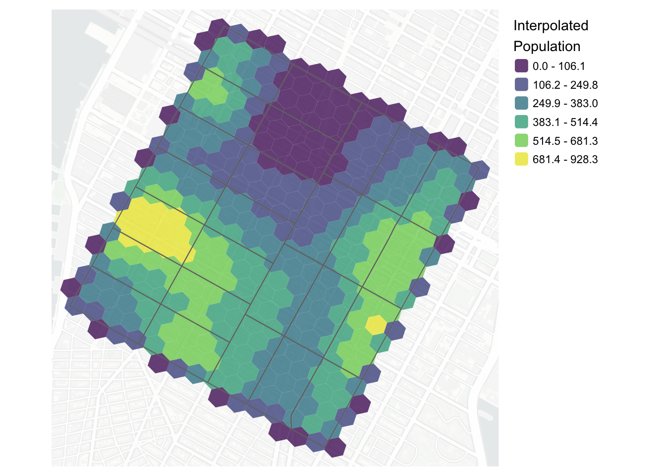
This example interpolates census tract population counts for a small area of New York City to an H3 grid at resolution 10:
out_nyc_ct_small <- nyc_ct_small |>
  pycnogrid::to_grid(
    value_col = populationE,
    grid_type = "h3",
    resolution = 10
  )
The returned object is an {sf} object containing the target-cell geometries, the interpolated count, an estimated density, and the proportion of each cell covered by the source geography. The map below shows the interpolated population counts:
Results for all census tracts in New York City at H3 resolution 9 can be generated using the code below:
out_nyc_ct <- nyc_ct |>
  pycnogrid::to_grid(
    value_col = populationE,
    grid_type = "h3",
    resolution = 9
  )
And mapped:
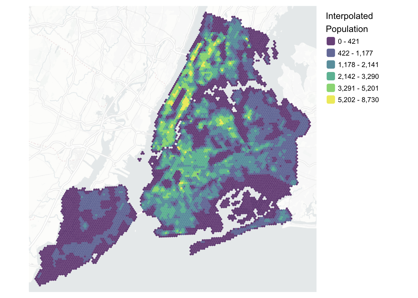
How did it do – does the sum of the interpolated population match the original total? Let’s see the interpolated results:
out_nyc_ct |>
  st_drop_geometry() |>
  summarize(total_pycno_populationE = sum(pycno_populationE)) |>
  pull(total_pycno_populationE)
[1] 8516202And the original census tract populations:
nyc_ct |>
  st_drop_geometry() |>
  summarize(total_populationE = sum(populationE)) |>
  pull(total_populationE)
[1] 8516202There we have it, {pycnogrid} provided a smoothed and mass-preserving pycnophylactic interpolation of population values from census tracts to, in this case, an H3 grid!
References
Brunsdon, Chris. 2025. Pycno: Pycnophylactic Interpolation. https://doi.org/10.32614/CRAN.package.pycno.
Eli Knaap, Renan Xavier Cortes, James Gaboardi, et al. 2026. Pysal/Tobler: V0.14.0. April 10. https://doi.org/10.5281/ZENODO.3386576.
Tobler, Waldo R. 1979. “Smooth Pycnophylactic Interpolation for Geographical Regions.” Journal of the American Statistical Association 74 (367): 519–30. https://doi.org/10.1080/01621459.1979.10481647.